Remote Sensing And Satellite Imagery

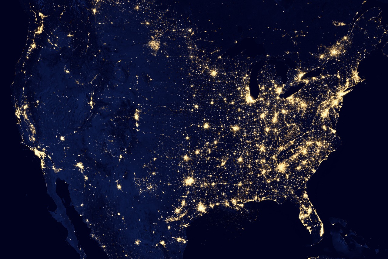
Remote sensing is the acquisition of information about the Earth’s atmosphere, land surface, and oceans from a distance, typically using instruments mounted on aircraft or satellites. In the context of weather prediction, remote sensing provides the observational backbone for initializing numerical models, validating forecasts, and monitoring atmospheric phenomena in near‑real time. The terminology used in this field is extensive, and a clear understanding of each term is essential for applying artificial intelligence techniques effectively. The following exposition defines the principal concepts, illustrates their practical use, and highlights the challenges that arise when integrating remote‑sensing data into AI‑driven weather prediction pipelines.

Electromagnetic spectrum The electromagnetic (EM) spectrum encompasses all wavelengths of electromagnetic radiation, ranging from gamma rays at sub‑nanometer scales to radio waves that can be many meters long. Weather‑relevant remote‑sensing instruments operate primarily in the visible (0.4–0.7 Μm), infrared (0.7–15 Μm), and microwave (1 mm–10 cm) portions of the spectrum. Each spectral band interacts differently with atmospheric gases, clouds, precipitation particles, and surface features, enabling the retrieval of distinct physical quantities. For example, the 6.7 Μm water‑vapor band is sensitive to mid‑tropospheric humidity, while the 10.7 Μm infrared window provides cloud‑top temperature information.

Spectral resolution Spectral resolution refers to the ability of a sensor to discriminate between adjacent wavelengths. High spectral resolution sensors, such as hyperspectral imagers, divide a spectral range into hundreds of narrow channels, each typically a few nanometers wide. This fine discrimination allows the identification of specific gases (e.G., Ozone, carbon dioxide) through absorption features. In contrast, multispectral sensors like the Moderate Resolution Imaging Spectroradiometer (MODIS) have a limited set of broader bands (e.G., 36 Channels ranging from 0.4 To 14.4 Μm). The choice of spectral resolution influences the type of AI models that can be trained; hyperspectral data provide richer feature spaces but demand larger computational resources and more sophisticated dimensionality‑reduction techniques.

Spatial resolution Spatial resolution describes the smallest ground area that can be distinguished by a sensor, usually expressed as the ground‑sample distance (GSD) or pixel size. A 1 km resolution product means each pixel represents a 1 km × 1 km area on the Earth’s surface. Higher spatial resolution (e.G., 250 M from the Visible Infrared Imaging Radiometer Suite, VIIRS) captures finer details such as convective storm cells, while coarser resolution (e.G., 25 Km from the Atmospheric Infrared Sounder, AIRS) is suitable for large‑scale temperature and humidity profiling. AI algorithms must account for the trade‑off between resolution and data volume; finer resolution provides more detailed inputs but can increase training time and memory consumption.

Temporal resolution Temporal resolution, or revisit time, is the interval between successive observations of the same location. Geostationary satellites, orbiting at roughly 35,786 km above the equator, offer high temporal resolution (as frequent as every 5 minutes for the GOES‑16 Advanced Baseline Imager, ABI). Polar‑orbiting satellites, such as the NOAA‑20, typically revisit a given point every 12 hours. High temporal resolution is critical for tracking rapidly evolving weather systems, and AI models that ingest time‑series data—such as recurrent neural networks (RNNs) or temporal convolutional networks—benefit from densely sampled observations.

Radiance Radiance (often denoted L) is the fundamental measurement recorded by satellite sensors. It represents the amount of electromagnetic energy traveling in a specific direction per unit area, per unit solid angle, per unit wavelength. Radiance values are usually expressed in watts per square meter per steradian per micrometer (W m⁻² sr⁻¹ µm⁻¹). Sensors convert incoming radiance into digital numbers (DN) through analog‑to‑digital conversion; calibration coefficients then translate DN to physical radiance units. AI pipelines typically ingest calibrated radiance or derived products (e.G., Brightness temperature) rather than raw DN to ensure physical consistency.

Brightness temperature Brightness temperature (T_B) is the temperature a blackbody would need to have to emit the observed radiance at a given wavelength, assuming the Rayleigh‑Jeans approximation holds. Infrared sensors commonly report data in brightness temperature units (Kelvin). Because real Earth surfaces and clouds are not perfect blackbodies, T_B is an indirect measure of physical temperature, modulated by emissivity and atmospheric absorption. Machine‑learning models often use brightness temperature as an input feature for cloud‑top temperature estimation, convective‑storm detection, and precipitation retrieval.

Reflectance Reflectance quantifies the fraction of incident solar radiation that is reflected by a surface or atmospheric constituent. In the visible and near‑infrared bands, satellite products are often expressed as either top‑of‑atmosphere (TOA) reflectance or surface reflectance after atmospheric correction. Reflectance values range from 0 (no reflection) to 1 (total reflection). Vegetation indices such as the Normalized Difference Vegetation Index (NDVI) are derived from reflectance in the red and near‑infrared bands; these indices can be incorporated into AI models to improve land‑surface temperature bias correction.

Radiometric resolution Radiometric resolution describes the sensor’s ability to discriminate small differences in radiance, typically expressed as the number of bits per pixel. An 8‑bit sensor can distinguish 256 discrete levels, while a 12‑bit sensor provides 4096 levels. Higher radiometric resolution improves the signal‑to‑noise ratio (SNR) and enables the detection of subtle atmospheric features, such as thin cirrus clouds. AI algorithms that operate on low‑bit data may require preprocessing steps like histogram equalization or noise reduction to avoid degrading model performance.

Signal‑to‑noise ratio (SNR) SNR is the ratio of the desired signal to the background noise, often expressed in decibels (dB). High SNR is essential for accurate retrievals; low SNR can obscure weak signals such as low‑level moisture gradients. In AI contexts, noisy inputs can lead to overfitting or poor generalization. Data‑augmentation techniques, denoising autoencoders, and robust loss functions are common strategies to mitigate the impact of sensor noise.

Calibration Calibration is the process of establishing a relationship between raw sensor output and physical units. It includes radiometric calibration (linking DN to radiance), spectral calibration (ensuring correct band central wavelengths), and geometric calibration (aligning pixels with geographic coordinates). Calibration can be performed on the ground (pre‑launch), in‑orbit using onboard blackbody references, or through vicarious methods that compare satellite observations with ground‑based measurements. Accurate calibration is a prerequisite for any AI‑driven assimilation or forecasting system because systematic biases can be amplified during model training.

Geolocation Geolocation determines the latitude and longitude of each pixel in a satellite image. It relies on precise knowledge of the satellite’s orbit (ephemeris data), sensor viewing geometry, and Earth‑rotation parameters. Errors in geolocation can lead to misalignment when fusing data from multiple sensors (e.G., Merging microwave and visible imagery). AI workflows that combine multi‑sensor datasets often employ regridding or interpolation onto a common grid; accurate geolocation minimizes interpolation error and preserves physical relationships.

Orbit types Two principal orbit configurations dominate weather‑satellite operations: Geostationary and polar‑orbiting (including low‑Earth orbit, LEO). Geostationary satellites maintain a fixed position relative to the Earth’s surface, providing continuous coverage of a specific region. Their high temporal resolution is advantageous for nowcasting and rapid‑update cycles. Polar‑orbiting satellites travel in near‑sun‑synchronous paths, crossing the equator at the same local solar time on each pass. This geometry yields consistent illumination conditions, facilitating the retrieval of surface‑based products such as land‑surface temperature. Understanding the strengths and limitations of each orbit type guides the selection of appropriate datasets for AI model training.

Sensor platforms Common weather‑satellite platforms include:

- GOES (Geostationary Operational Environmental Satellite) series: GOES‑16 and GOES‑17 provide full‑disk imaging every 10 minutes, with mesoscale sectors every 5 minutes. Their ABI instrument offers 16 spectral bands, spanning visible to infrared. - METOP (Meteorological Operational satellite) series: METOP‑A, B, and C carry the Advanced Microwave Sounding Unit (AMSU) and the Infrared Atmospheric Sounding Interferometer (IASI). These sensors deliver temperature and humidity profiles with vertical resolution. - NOAA (National Oceanic and Atmospheric Administration) polar‑orbiting series: NOAA‑20 (JPSS‑1) hosts the VIIRS and CrIS (Cross‑track Infrared Sounder) instruments, providing high‑resolution visible/infrared data and hyperspectral soundings. - Himawari series (Japan): Himawari‑8 and Himawari‑9 deliver rapid‑scan imagery over the Asia‑Pacific region, with 5‑minute full‑disk updates. - Sentinel series (European Space Agency): Sentinel‑3 carries the Sea and Land Surface Temperature Radiometer (SLSTR) and the Ocean and Land Colour Instrument (OLCI), useful for marine‑atmospheric coupling studies.

Each platform presents a distinct set of bands, resolutions, and data volumes, influencing the design of AI pipelines. For instance, training a convolutional neural network (CNN) to detect tropical cyclones may benefit from the high‑frequency visible/infrared data of Himawari, while a data‑assimilation system that requires upper‑tropospheric temperature profiles may rely on IASI hyperspectral retrievals.

Radiative transfer Radiative transfer describes the propagation of electromagnetic radiation through the atmosphere, accounting for absorption, emission, and scattering by gases, aerosols, and cloud particles. Forward radiative‑transfer models (e.G., RTTOV, MODTRAN) simulate sensor radiances given atmospheric state variables, while inverse models retrieve atmospheric profiles from observed radiances. AI techniques increasingly replace or augment traditional inversion methods; for example, neural‑network‑based retrievals can approximate the inverse radiative‑transfer operator with reduced computational cost. Nevertheless, a solid grasp of radiative‑transfer physics remains essential to interpret model outputs and to enforce physical consistency during training.

Cloud masking Cloud masking identifies pixels that contain clouds, which is a prerequisite for many surface‑based products. Simple threshold‑based algorithms use brightness temperature differences (e.G., Between 11 µm and 12 µm channels) to flag cloud presence. More sophisticated approaches employ machine‑learning classifiers that combine multiple spectral features, texture metrics, and temporal context. Accurate cloud masks improve the reliability of AI‑driven precipitation retrievals and surface temperature estimates. Challenges include distinguishing thin cirrus from clear sky and handling mixed‑pixel conditions at coarse resolutions.

Precipitation retrieval Precipitation retrievals translate satellite radiances into quantitative rain‑rate estimates. Infrared‑only methods infer rain intensity from cloud‑top temperature, assuming a relationship between colder clouds and stronger convection. Microwave‑based techniques, such as those using the Advanced Microwave Scanning Radiometer (AMSR‑2), directly sense scattering and emission from raindrops and ice particles, providing more accurate surface rain rates. Hybrid algorithms blend infrared and microwave data. AI models, particularly deep learning architectures, have shown promise in fusing multi‑sensor inputs to produce high‑resolution precipitation maps. However, validation against ground‑based radar and gauge networks remains a critical step.

Data assimilation Data assimilation (DA) integrates observations into numerical weather prediction (NWP) models to produce an analysis that best represents the atmospheric state. Classic DA methods, such as three‑dimensional variational (3D‑Var) and four‑dimensional variational (4D‑Var), minimize a cost function that balances observation and background errors. Recent research explores the use of AI to approximate the DA operator, accelerate the minimization process, or learn error covariance structures. Understanding the observational error characteristics of remote‑sensing products is vital for any AI‑enhanced DA system.

Geophysical variables Remote‑sensing observations are often converted into geophysical variables that are directly usable by NWP models. Common variables include:

- Temperature (T) at various pressure levels - Specific humidity (q) - Wind components (u, v) derived from cloud‑track wind algorithms - Surface pressure (p_s) - Cloud‑fraction (CF) and cloud‑optical‑depth (COD) - Aerosol optical depth (AOD)

AI models may predict these variables directly from satellite radiances (end‑to‑end learning) or ingest pre‑processed products. The choice depends on the availability of training labels, computational constraints, and the desired level of physical interpretability.

Level‑2 and Level‑3 products Satellite data are categorized into processing levels. Level‑0 is raw telemetry; Level‑1 contains calibrated radiances and geolocation; Level‑2 provides geophysical retrievals (e.G., Temperature profiles); Level‑3 aggregates data onto a regular grid, often with temporal averaging. For AI applications, Level‑2 products are attractive because they reduce the need for complex retrieval algorithms, while Level‑3 products facilitate spatial alignment across sensors. Nevertheless, Level‑2 retrievals may embed algorithmic biases that must be accounted for during model training.

Bias correction Bias correction adjusts systematic differences between observed and modeled quantities. In satellite remote sensing, biases arise from sensor calibration drift, algorithmic approximations, and mismatches between model and observation resolutions. Statistical bias‑correction methods (e.G., Quantile mapping) are widely used, but AI offers data‑driven alternatives, such as conditional generative adversarial networks (cGANs) that learn to transform biased fields into unbiased counterparts. Effective bias correction improves the compatibility of satellite data with NWP models and enhances forecast skill.

Data volume and storage Modern weather satellites generate terabytes of data per day. For instance, GOES‑16 ABI produces roughly 1.5 TB of Level‑1B data daily. Managing such volumes requires efficient storage formats (e.G., NetCDF4, HDF5), compression, and parallel I/O. AI training pipelines must be designed to stream data from disk, use mini‑batching, and leverage distributed computing resources. Cloud‑based storage and processing platforms (e.G., AWS S3 with EC2 GPU instances) are increasingly adopted to handle the data deluge.

Pre‑processing steps Typical pre‑processing stages include:

1. Calibration from DN to radiance. 2. Geolocation and projection onto a common map projection (e.G., Geostationary‑satellite projection, latitude‑longitude grid). 3. Cloud‑mask application. 4. Temporal interpolation or aggregation to the desired analysis time. 5. Resampling to a uniform spatial resolution (e.G., 0.5° × 0.5° For global models). 6. Normalization (e.G., Min‑max scaling) to improve neural‑network convergence.

Each step introduces potential sources of error; AI practitioners must document and, where possible, quantify these uncertainties.

Feature engineering Although deep learning reduces the need for manual feature design, many remote‑sensing applications still benefit from engineered features that capture physical relationships. Examples include:

- Brightness‑temperature differences (BTD) between water‑vapor and infrared channels to highlight moisture gradients. - Texture metrics such as the Gray‑Level Co‑Occurrence Matrix (GLCM) applied to visible bands for cloud‑type discrimination. - Spatial gradients (e.G., ∇T) to identify frontal zones. - Temporal differencing (ΔT) to detect rapid cooling associated with convective initiation.

These engineered features can be concatenated with raw spectral inputs, providing the model with both low‑level and high‑level information.

Training labels Supervised learning requires ground‑truth labels. In weather remote sensing, labels may come from:

- Radar reflectivity fields (e.G., NEXRAD) for precipitation classification. - In‑situ observations from radiosondes for temperature and humidity profiles. - Reanalysis datasets (e.G., ERA5) that assimilate a broad suite of observations. - Human‑annotated storm tracks for tropical‑cyclone detection.

Label quality, spatial representativeness, and temporal alignment are critical. Misaligned labels can degrade model performance, especially when the satellite observation and the reference dataset have differing resolutions or observation times.

Evaluation metrics Assessing AI models that ingest remote‑sensing data involves a range of statistical metrics, selected according to the target variable:

- Mean Absolute Error (MAE) and Root Mean Square Error (RMSE) for continuous fields (e.G., Temperature). - Critical Success Index (CSI) and Equitable Threat Score (ETS) for categorical events such as convective‑storm detection. - Receiver Operating Characteristic (ROC) curves and Area Under the Curve (AUC) for binary classification (e.G., Cloud vs. Clear). - Continuous Ranked Probability Score (CRPS) for probabilistic forecasts generated by ensemble AI methods.

Consistent use of these metrics enables fair comparison between traditional physics‑based retrievals and AI‑driven alternatives.

Domain adaptation Satellite sensors evolve over time; new generations may have different spectral channels, improved calibration, or altered viewing geometries. AI models trained on legacy data may underperform on newer observations due to domain shift. Domain‑adaptation techniques—such as fine‑tuning on a small set of recent data, adversarial training to learn sensor‑invariant representations, or using synthetic data generated by radiative‑transfer simulations—help maintain model relevance across sensor upgrades.

Uncertainty quantification Weather prediction inherently involves uncertainty. AI models can incorporate uncertainty estimates through:

- Monte Carlo dropout, where dropout layers are kept active during inference to generate an ensemble of predictions. - Bayesian neural networks that learn posterior distributions over weights. - Ensembles of independently trained models, whose spread reflects predictive confidence. - Probabilistic loss functions (e.G., Negative log‑likelihood) that encourage the model to output predictive distributions rather than point estimates.

Quantifying uncertainty is especially important when satellite observations are used to trigger high‑impact weather warnings.

Explainability and interpretability Stakeholders demand transparent AI systems, particularly in operational forecasting where decision‑makers rely on model outputs. Techniques such as saliency maps, Grad‑CAM, and SHAP values can highlight which spectral channels or spatial regions most influence a model’s prediction. For remote‑sensing applications, explainability helps verify that the AI model is responding to physically meaningful patterns—e.G., Focusing on cold cloud tops for severe‑storm detection rather than spurious sensor noise.

Multi‑sensor fusion Combining data from disparate sensors enhances the information content available to AI models. Common fusion strategies include:

- Early fusion: Stacking radiances from different sensors as separate channels in the input tensor. - Late fusion: Processing each sensor’s data through separate subnetworks and merging the learned representations before the final prediction layer. - Hybrid fusion: Integrating both low‑level pixel information and high‑level derived products (e.G., Blending brightness temperature with cloud‑fraction fields).

Challenges in multi‑sensor fusion involve aligning temporal and spatial sampling, handling missing data (e.G., Due to sensor outages), and reconciling differing noise characteristics.

Geophysical consistency constraints Pure data‑driven models may produce physically inconsistent outputs—such as temperature profiles that violate the hydrostatic balance. To enforce realism, AI frameworks can embed physical constraints directly into the loss function (e.G., Penalizing negative humidity values) or employ physics‑informed neural networks (PINNs) that incorporate governing equations as part of the training process. This approach improves generalization, especially when extrapolating to unseen atmospheric regimes.

Operational considerations Deploying AI models in an operational weather center entails several practical aspects:

- Latency: The model must deliver predictions within the time window required for rapid‑update cycles (e.G., < 5 Minutes for nowcasting). - Robustness: The system should handle data gaps, sensor anomalies, and out‑of‑distribution events without crashing. - Scalability: Parallel processing on GPUs or distributed clusters is often necessary to ingest high‑frequency satellite streams. - Verification: Continuous performance monitoring against benchmark datasets ensures that model degradation is detected early.

Integration with existing DA pipelines, such as the Earth System Modeling Framework (ESMF), often requires wrapper scripts that translate AI outputs into model‑compatible formats.

Case study: AI‑enhanced convective‑storm detection Consider a CNN trained on GOES‑16 ABI visible (0.47 Μm) and infrared (10.3 Μm) channels to identify nascent convective cells. The workflow includes:

1. Retrieval of Level‑1B radiances for a 30‑minute window. 2. Application of a cloud mask to exclude clear‑sky pixels. 3. Calculation of the brightness‑temperature difference between the 10.3 Μm and 11.2 Μm channels, which highlights water‑vapor absorption. 4. Stacking the original visible radiance, the BTD map, and the cloud‑mask as a three‑channel input tensor. 5. Training the CNN with labels derived from NEXRAD radar reflectivity, using a threshold of 35 dBZ to define storm cells. 6. Evaluating the model with CSI and AUC, achieving a CSI improvement of 12 % over the baseline threshold‑based algorithm. 7. Deploying the model in a real‑time pipeline that ingests ABI data every 5 minutes, generates storm‑cell probability maps, and forwards alerts to the warning center.

Key challenges observed in this case include handling the varying illumination conditions near sunrise/sunset, which affect visible radiance, and mitigating false alarms caused by bright surface features (e.G., Deserts). Incorporating a temporal RNN layer helped the model learn the evolution of cloud features, reducing spurious detections.

Case study: Neural‑network retrieval of atmospheric temperature profiles A fully connected network (FCN) is trained to emulate the inverse of the RTTOV radiative‑transfer model. Input features consist of brightness temperatures from 15 infrared channels of the IASI instrument. The target is the temperature profile at 21 pressure levels. The training dataset is generated by forward‑modeling a large ensemble of atmospheric states sampled from ERA5. After training, the FCN provides temperature profiles in milliseconds, a factor of 100 faster than traditional optimal‑estimation methods. Validation against independent radiosonde launches shows a root‑mean‑square error of 1.2 K in the mid‑troposphere, comparable to the operational IASI retrieval. However, the FCN struggles with extreme temperature inversions, highlighting the need for incorporating additional constraints or hybridizing with physics‑based retrievals.

Case study: Data assimilation with AI‑generated observation operators In a 4D‑Var DA system, the observation operator maps model state variables to simulated satellite radiances. A deep‑learning surrogate for the observation operator is trained on a large set of model states and corresponding RTTOV‑generated radiances. During assimilation, the surrogate replaces the expensive radiative‑transfer call, reducing the cost of the cost‑function gradient calculation by 70 %. Experiments demonstrate that the analysis increment obtained with the surrogate is nearly identical to that from the full physics operator, provided the surrogate is periodically retrained to capture model changes. This example illustrates how remote‑sensing vocabulary (e.G., “Radiance,” “brightness temperature”) translates into concrete AI components that accelerate core forecasting workflows.

Challenges specific to AI and remote sensing

1. Data heterogeneity: Satellite instruments differ in spectral coverage, resolution, and noise characteristics. Harmonizing these heterogeneous datasets for AI training demands careful preprocessing and often bespoke model architectures.

2. Label scarcity: High‑quality ground truth is limited, especially over oceans and sparsely populated regions. Semi‑supervised learning, self‑training, and transfer learning are active research areas to mitigate label paucity.

3. Physical interpretability: Deep networks can be “black boxes,” making it difficult to ensure that predictions respect fundamental atmospheric physics. Embedding constraints or using hybrid physics‑machine‑learning models addresses this concern.

4. Computational demand: The volume of satellite data, combined with the size of modern neural networks, results in substantial compute requirements. Efficient data pipelines, mixed‑precision training, and model compression (e.G., Pruning, quantization) are essential for operational feasibility.

5. Real‑time processing: Weather forecasting imposes strict latency limits. AI models must be optimized for inference speed, possibly via model distillation or deployment on specialized hardware (e.G., Tensor Processing Units).

6. Sensor degradation: Over a satellite’s lifespan, sensor performance may drift. Continuous monitoring of calibration and adaptive retraining of AI models are required to maintain accuracy.

7. Regulatory and ethical considerations: The use of AI in public‑safety forecasting raises questions about accountability, transparency, and equitable access to improved forecasts. Clear documentation of model provenance and performance is mandatory.

Future directions

The convergence of remote sensing and AI is poised to transform weather prediction. Emerging trends include:

- End‑to‑end learning that maps raw satellite radiances directly to forecast fields, bypassing intermediate retrieval steps. - Self‑supervised pretraining on massive archives of satellite imagery, analogous to language‑model pretraining, to learn universal atmospheric representations. - Coupled ocean‑atmosphere AI models that ingest both atmospheric satellite data and oceanic remote‑sensing products (e.G., Sea‑surface temperature, sea‑ice concentration) for integrated forecasting. - Hybrid DA frameworks that blend AI‑generated increments with traditional variational methods, leveraging the strengths of both. - Explainable AI dashboards that present model reasoning alongside conventional meteorological diagnostics, fostering trust among forecasters.

By mastering the terminology outlined above, students and practitioners can navigate the complex landscape of satellite remote sensing, design robust AI pipelines, and contribute to the next generation of high‑impact weather prediction systems.