Advanced Statistical Methods For Forecasting

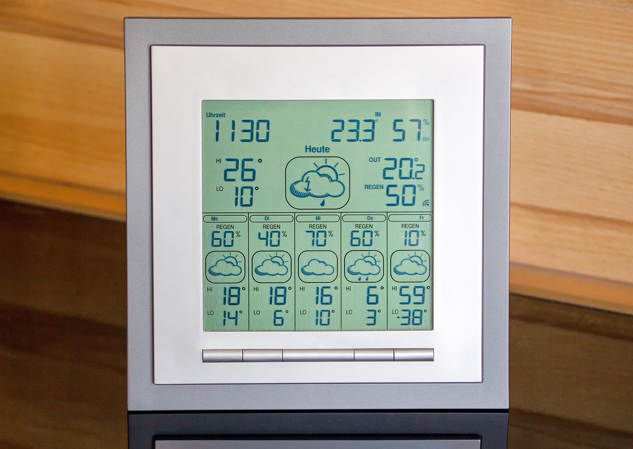
Time series data are sequences of observations collected at regular time intervals. In weather prediction, typical time series include hourly temperature, daily precipitation totals, or monthly wind speed averages. Understanding the temporal structure of these series is fundamental because many statistical forecasting models, such as autoregressive processes, rely on the assumption that past values contain information about future values. A simple example is a temperature record from a coastal station: The temperature at 10 am today is often strongly correlated with the temperature at 9 am, reflecting the persistence of atmospheric conditions.

Autoregressive (AR) model describes a time series where the current value is expressed as a linear combination of its previous values plus a random error term. The model order, denoted AR(p), indicates how many lagged observations are used. For instance, an AR(2) model for daily maximum temperature might be written as T_t = φ_1 T_{t‑1} + φ_2 T_{t‑2} + ε_t, where φ_1 and φ_2 are coefficients estimated from historical data and ε_t is a white‑noise error. In practice, fitting an AR model to a temperature series helps capture short‑term persistence, which is useful for forecasts up to a few days.

Moving average (MA) model complements the AR approach by modeling the current observation as a function of past forecast errors. An MA(q) model uses q lagged error terms: X_t = μ + θ_1 ε_{t‑1} + … + θ_q ε_{t‑q} + ε_t. The combination of AR and MA components yields the ARMA model, which is appropriate for stationary series where the mean and variance do not change over time. Weather variables often exhibit non‑stationarity due to seasonality; therefore, transformations such as differencing are applied before fitting ARMA models.

Integrated (I) component refers to the number of differencing operations required to achieve stationarity. The classic ARIMA (AutoRegressive Integrated Moving Average) model is denoted ARIMA(p,d,q), where d is the order of differencing. For example, a monthly precipitation series may show a strong seasonal cycle; differencing the series once (d = 1) often removes the trend, allowing the ARMA part to model the remaining stochastic variation.

Seasonal ARIMA (SARIMA) extends ARIMA by incorporating seasonal terms. The full notation SARIMA(p,d,q)(P,D,Q)_s includes seasonal autoregressive (P), seasonal differencing (D), and seasonal moving‑average (Q) terms, with s indicating the seasonal period (e.G., 12 For monthly data). A SARIMA(1,1,1)(0,1,1)_12 model could be used to forecast monthly rainfall, where the seasonal differencing removes the annual cycle and the seasonal MA term captures the residual seasonal autocorrelation.

State‑space representation provides a flexible framework for modeling dynamic systems. In this formulation, the observed variable y_t is linked to an unobserved state vector x_t through an observation equation y_t = H x_t + v_t, while the state evolves according to x_t = F x_{t‑1} + w_t. Matrices H and F define the observation and transition relationships, respectively, and v_t and w_t are error terms. This structure underlies many advanced filtering techniques, such as the Kalman filter, and enables the incorporation of physical constraints from numerical weather prediction (NWP) models.

Kalman filter is an optimal recursive algorithm for estimating the hidden state of a linear Gaussian system. At each time step it performs a prediction based on the transition model and then updates the estimate using the new observation, minimizing the mean‑square error. In weather forecasting, Kalman filters are employed for data assimilation, where observations from satellites, radars, and surface stations are merged with NWP model outputs to produce an improved analysis of the atmospheric state. The filter’s ability to quantify uncertainty through error covariance matrices is critical for subsequent probabilistic forecasts.

Extended Kalman filter (EKF) generalizes the Kalman filter to handle non‑linear dynamics by linearizing the transition and observation functions around the current estimate. Although EKF can be applied to atmospheric variables that evolve non‑linearly, the linearization may introduce bias, especially during extreme events such as rapid cyclogenesis. Consequently, more robust alternatives like the particle filter are often preferred for highly non‑linear applications.

Particle filter, also known as Sequential Monte Carlo, approximates the posterior distribution of the state by a set of weighted particles. Each particle represents a possible realization of the atmospheric state, and weights are updated based on the likelihood of the observed data. This approach can capture multi‑modal distributions and strong non‑linearities, making it suitable for forecasting severe weather where multiple plausible scenarios coexist. The main challenge lies in computational cost, as a large number of particles is required to avoid sample impoverishment in high‑dimensional atmospheric spaces.

Ensemble Kalman filter (EnKF) combines the Kalman filter’s statistical framework with Monte‑Carlo sampling. An ensemble of model forecasts is propagated forward, and the sample covariance of the ensemble serves as an estimate of the error covariance. The EnKF is widely used in operational weather centers because it scales better to the thousands of state variables in a typical NWP model while still providing a probabilistic description of forecast uncertainty.

Variational data assimilation formulates the analysis problem as the minimization of a cost function that measures the misfit between the model state and observations, weighted by their respective error covariances. The most common implementations are three‑dimensional variational (3D‑Var) and four‑dimensional variational (4D‑Var) assimilation. 3D‑Var assumes observations are instantaneous, whereas 4D‑Var incorporates observations over a time window, effectively accounting for the model dynamics during the assimilation interval. The gradient of the cost function is obtained using an adjoint model, which is the transpose of the linearized forward model.

Adjoint model computes the sensitivity of a scalar cost function to the model state by propagating information backward in time. In the context of 4D‑Var, the adjoint provides the gradient needed for iterative minimization. Developing an accurate adjoint for a complex atmospheric model is a major engineering effort, but it enables the assimilation of large volumes of satellite radiances and radar reflectivity, improving forecast skill at medium ranges.

Background error covariance (often denoted B) quantifies the uncertainty of the prior (background) state before assimilation. Accurate specification of B is essential because it determines how much weight the observations receive relative to the model forecast. In practice, B is estimated from historical forecast errors, ensemble statistics, or climatological variances. Spatially varying B can capture differences in predictability, such as greater uncertainty in the tropics compared with mid‑latitudes.

Observation operator (denoted H) maps model variables to observation space. For satellite radiances, H involves a radiative transfer model that converts temperature and moisture profiles into brightness temperatures. Linearizing H yields the Jacobian matrix, which is required in variational methods and the EKF. Errors in the observation operator propagate directly into analysis errors, so careful validation against ground truth is necessary.

Analysis refers to the best estimate of the atmospheric state after combining observations with the background. In operational centers, the analysis is the starting point for the forecast integration. The quality of the analysis is typically assessed by independent observations not used in the assimilation, such as radiosonde data withheld for validation.

Forecast cycle denotes the sequence of steps from data assimilation, model integration, to post‑processing and verification. A typical 12‑hour cycle may involve ingesting observations at 00 UTC and 12 UTC, generating a 0‑day analysis, running the NWP model forward to produce forecasts out to 72 hours, and then applying statistical post‑processing techniques such as bias correction or probabilistic calibration.

Reanalysis products are generated by repeatedly assimilating historical observations into a consistent model framework, creating a uniform climate dataset. The ERA5 reanalysis, for example, provides hourly fields of temperature, wind, and humidity back to 1979. Researchers use reanalysis data to train statistical forecasting models, evaluate long‑term trends, and develop climate indices.

Hindcasting involves running a forecast model retrospectively using past observations to evaluate its performance. Hindcasts are essential for assessing the skill of new statistical methods before operational deployment. By comparing hindcast ensembles against known outcomes, analysts can quantify forecast reliability, bias, and uncertainty.

Lead time is the interval between the analysis time and the forecast valid time. Forecast skill generally decays with increasing lead time due to error growth in the atmospheric dynamics. Statistical methods often target specific lead times; for example, a nowcasting system may focus on 0‑6 hour forecasts of precipitation, while medium‑range models aim for 3‑day predictions.

Probabilistic forecasting provides a distribution of possible outcomes rather than a single deterministic value. In weather prediction, this is expressed as forecast probabilities for events such as “rain > 10 mm in the next 24 hours.” Probabilistic forecasts enable decision makers to weigh risks and benefits, for instance, in aviation or agriculture. Techniques for generating probabilistic forecasts include ensemble methods, Bayesian inference, and post‑processing of deterministic model output.

Deterministic forecast supplies a single best‑guess value, often the ensemble mean or the control run of an NWP model. While deterministic forecasts are intuitive, they hide the underlying uncertainty and can be misleading when the spread is large. Many operational centers now supplement deterministic outputs with probabilistic information to provide a fuller picture.

Bias correction adjusts systematic errors in model forecasts. A common approach is to compute the mean error of past forecasts for a given location and season, then subtract this bias from future forecasts. For temperature, a simple additive correction may suffice; for precipitation, multiplicative or quantile‑mapping techniques are often required because precipitation errors are highly skewed.

Post‑processing encompasses a suite of statistical techniques applied after the raw model output to improve accuracy, reliability, and usability. Methods include regression‑based correction, analog forecasting, machine‑learning ensembles, and probabilistic calibration. Effective post‑processing can significantly increase forecast skill, especially for variables with complex error structures such as convective precipitation.

Statistical downscaling translates coarse‑resolution model output to finer scales using statistical relationships derived from historical observations. For example, a regional climate model providing 50 km temperature fields can be downscaled to 5 km using a regression model that relates large‑scale predictors (e.G., Geopotential height) to local temperature. Downscaling is valuable for impact studies that require high‑resolution information, such as flood risk assessment.

Dynamical downscaling involves nesting a high‑resolution NWP model within a coarser global model. The fine‑scale model receives boundary conditions from the parent model, allowing it to resolve mesoscale phenomena like mountain waves or sea‑breeze circulations. While more computationally demanding than statistical downscaling, dynamical downscaling retains physical consistency and can capture non‑linear interactions.

Model error denotes the discrepancy between the true atmospheric evolution and the model’s representation of it. Sources include imperfect physical parameterizations, discretization errors, and neglected processes. Model error is often treated as a stochastic term in statistical forecasting, leading to techniques such as model error covariance estimation or stochastic physics schemes.

Observation error arises from instrument inaccuracies, representativeness mismatch, and preprocessing steps. For satellite radiances, calibration uncertainties and cloud contamination contribute to observation error. Accurate error characterization is crucial for data assimilation because it determines the relative trust placed in observations versus the background.

Uncertainty quantification aims to characterize the range of plausible forecast outcomes. In statistical forecasting, uncertainty is expressed through confidence intervals, prediction intervals, or full probability density functions. For example, a 90 % prediction interval for tomorrow’s maximum temperature may be 22 °C – 28 °C, indicating that the true temperature is expected to fall within this range with 90 % confidence.

Confidence interval provides a range around a point estimate (e.G., The mean forecast) within which the true parameter lies with a given probability. In regression‑based temperature forecasting, a 95 % confidence interval around the regression line indicates the uncertainty of the estimated relationship.

Prediction interval differs from a confidence interval by accounting for both parameter uncertainty and the inherent randomness of future observations. It is therefore wider and more appropriate for communicating forecast uncertainty to end users.

Bootstrapping is a resampling technique used to estimate the sampling distribution of a statistic by repeatedly drawing samples with replacement from the original dataset. In weather forecasting, bootstrapping can generate ensembles of regression coefficients, providing an empirical measure of forecast uncertainty without assuming normality.

Bagging (Bootstrap Aggregating) builds multiple models on bootstrap‑sampled subsets of the training data and aggregates their predictions, typically by averaging. Bagging reduces variance and improves stability, especially for high‑variance learners such as decision trees. Random Forests are a classic example of bagging applied to tree ensembles.

Boosting sequentially fits models to the residuals of previous models, emphasizing difficult cases. Gradient boosting machines (GBMs) and XGBoost have become popular for weather prediction tasks such as precipitation classification because they can capture complex non‑linear relationships while controlling over‑fitting through regularization.

Random forest constructs an ensemble of decision trees using random subsets of predictors and data points. The randomness decorrelates the trees, leading to robust predictions and built‑in measures of variable importance. For example, a random forest may be trained to predict the probability of severe thunderstorms using predictors such as convective available potential energy (CAPE), moisture flux, and wind shear.

Gradient boosting iteratively adds weak learners that correct the errors of the ensemble so far. The method minimizes a differentiable loss function, allowing customized objectives such as quantile loss for probabilistic precipitation forecasts. XGBoost extends gradient boosting with regularization, parallel computation, and handling of missing values, making it suitable for large meteorological datasets.

Hyperparameter tuning involves searching for the optimal configuration of model settings that are not learned directly from the data (e.G., Number of trees, learning rate, maximum depth). Common strategies include grid search, random search, and Bayesian optimization. Proper tuning can substantially improve forecast skill, but excessive tuning may lead to overfitting on the validation set.

Cross‑validation partitions the data into training and validation subsets multiple times to assess model generalization. In the context of time‑series data, simple random splits can violate temporal dependencies; therefore, techniques such as rolling‑origin or blocked cross‑validation are preferred. For seasonal precipitation forecasting, a blocked scheme that respects yearly cycles prevents leakage of future information into the training set.

Overfitting occurs when a model captures noise rather than the underlying signal, leading to poor performance on unseen data. Regularization methods such as ridge regression, lasso, and elastic net penalize model complexity, reducing the risk of overfitting. In weather prediction, overfitting is a particular concern when using high‑resolution satellite data combined with many derived features.

Ridge regression adds an L2 penalty (λ ∑β_i^2) to the ordinary least‑squares loss, shrinking coefficient estimates toward zero. This stabilizes estimates in the presence of multicollinearity among predictors, a common situation when atmospheric variables are strongly correlated (e.G., Temperature and humidity).

Lasso (Least Absolute Shrinkage and Selection Operator) imposes an L1 penalty (λ ∑|β_i|), which can set some coefficients exactly to zero, performing variable selection. Lasso is useful for identifying the most informative predictors for a given forecast, such as selecting a subset of pressure‑level variables that best explain surface precipitation.

Elastic net combines L1 and L2 penalties, balancing variable selection and coefficient shrinkage. It is particularly effective when predictors are numerous and highly correlated, as is often the case with gridded reanalysis fields.

Feature engineering creates informative variables from raw data to improve model performance. In weather forecasting, typical engineered features include lagged variables, moving averages, diurnal cycles, and derived quantities like CAPE, lifted index, or wind shear. Proper feature engineering can capture physical processes that raw predictors alone may not reveal.

Principal component analysis (PCA) reduces dimensionality by projecting the data onto orthogonal directions of maximal variance. In atmospheric science, the technique is often referred to as Empirical Orthogonal Function (EOF) analysis. By retaining the leading EOFs, one can compress a high‑dimensional field (e.G., Geopotential height) into a few modes that capture the dominant large‑scale patterns, facilitating statistical modeling.

EOF analysis is synonymous with PCA applied to spatial fields. For example, the first EOF of sea‑level pressure may represent the North Atlantic Oscillation pattern, which is a powerful predictor of winter precipitation in Europe. Incorporating EOF scores as regressors in a statistical forecast model can improve skill by leveraging large‑scale teleconnections.

Dimensionality reduction techniques, such as PCA, autoencoders, or random projection, are essential when dealing with high‑resolution gridded datasets that contain millions of variables. Reducing dimensionality mitigates the curse of dimensionality, speeds up model training, and helps avoid overfitting.

Clustering groups similar observations together based on a chosen distance metric. Methods such as k‑means, hierarchical clustering, or Gaussian mixture models can segment weather regimes, enabling regime‑dependent forecasting. For instance, clustering of atmospheric circulation patterns may reveal distinct “blocking” and “zonal” regimes, each with its own precipitation characteristics.

k‑means clustering partitions the data into k clusters by minimizing within‑cluster variance. When applied to daily geopotential height fields, k‑means can identify recurring synoptic patterns that serve as predictors for subsequent precipitation forecasts.

Hierarchical clustering builds a tree of clusters by iteratively merging or splitting groups based on similarity. The dendrogram can reveal natural groupings without pre‑specifying the number of clusters, useful for exploratory analysis of atmospheric regimes.

Forecast verification assesses the quality of predictions using statistical metrics. Verification distinguishes between deterministic and probabilistic skill, evaluating attributes such as accuracy, reliability, resolution, and discrimination. Proper verification is essential for communicating forecast performance to stakeholders and for model improvement.

Skill scores quantify forecast quality relative to a reference, often climatology or a persistence forecast. Common skill scores include the Brier skill score for binary events, the continuous ranked probability score (CRPS) skill score for probabilistic forecasts, and the anomaly correlation coefficient for temperature anomalies.

Brier score measures the mean squared error of probability forecasts for binary events. A lower Brier score indicates better calibration and resolution. For example, forecasting a 30 % chance of rain that materializes 30 % of the time yields a perfect Brier score of zero, whereas consistently over‑confident forecasts increase the score.

Continuous ranked probability score (CRPS) evaluates the quality of a full predictive distribution by integrating the squared difference between the forecast CDF and the observation indicator function. CRPS reduces to the absolute error for deterministic forecasts, making it a versatile metric for comparing deterministic and probabilistic methods.

Reliability diagram plots observed frequencies against forecast probabilities, revealing calibration. A well‑calibrated forecast lies on the diagonal. In practice, precipitation probability forecasts often exhibit over‑confidence; reliability diagrams help identify and correct such biases through post‑processing.

Quantile mapping aligns the distribution of model forecasts with that of observations by matching quantiles. This non‑parametric bias correction technique is especially useful for variables with skewed distributions, such as daily precipitation totals. By applying quantile mapping, a model’s tendency to underestimate heavy rain events can be mitigated.

Probabilistic calibration adjusts forecast probabilities to improve reliability while preserving discrimination. Techniques include logistic regression (also known as reliability regression) and isotonic regression. Calibration is a critical step before issuing probabilistic forecasts to end users, ensuring that a stated 70 % chance of rain truly corresponds to a 70 % observed frequency over many cases.

Extreme value theory (EVT) provides statistical tools for modeling the tail behavior of distributions, essential for forecasting rare events such as severe thunderstorms or flash floods. The Generalized Extreme Value (GEV) distribution and the Generalized Pareto Distribution (GPD) are commonly employed to estimate return periods and exceedance probabilities.

Generalized Autoregressive Conditional Heteroskedasticity (GARCH) models time‑varying volatility, capturing periods of high variability in variables like wind speed. By modeling the conditional variance, GARCH can improve probabilistic forecasts of wind power generation, where variability directly impacts energy supply.

Spatial autocorrelation describes the tendency for nearby locations to exhibit similar values. Metrics such as Moran’s I quantify the degree of spatial dependence. Accounting for spatial autocorrelation is crucial when developing statistical models that use gridded observations, as ignoring it can lead to underestimated uncertainties.

Moran’s I ranges from –1 (perfect dispersion) to +1 (perfect clustering). A high positive Moran’s I for temperature fields indicates that neighboring grid points share similar values, justifying the use of spatial smoothing or kriging techniques.

Geostatistics encompasses statistical methods for spatial interpolation and prediction. Kriging, a best‑linear‑unbiased estimator, uses a variogram model to describe spatial dependence and provides both predictions and associated uncertainties. In meteorology, kriging can fill gaps in surface observations, producing high‑resolution temperature fields for model initialization.

Variogram characterizes how the variance between pairs of observations changes with separation distance. Fitting a variogram model (e.G., Spherical, exponential) allows the kriging algorithm to weight observations appropriately based on their spatial proximity.

Kriging produces an interpolated field that honors the observed data and the underlying spatial correlation structure. Ordinary kriging assumes a constant mean, while universal kriging incorporates a deterministic trend (e.G., Elevation). For mountainous regions, universal kriging can capture the lapse rate of temperature with altitude.

Anisotropy occurs when spatial correlation differs with direction, often due to prevailing wind patterns or topographic alignment. Incorporating anisotropy into the variogram improves interpolation accuracy for variables like wind speed, which may be more strongly correlated along the prevailing wind direction.

Covariance matrix captures the pairwise covariances among a set of variables. In data assimilation, the background error covariance matrix B is a large, often sparse, representation of forecast uncertainties. Efficient storage and inversion of such matrices rely on techniques like the Cholesky decomposition.

Precision matrix is the inverse of the covariance matrix, encoding conditional independence relationships. Sparse precision matrices arise in Gaussian Markov random fields, enabling scalable inference for high‑dimensional spatial fields.

Cholesky decomposition factorizes a positive‑definite matrix into a lower‑triangular matrix L such that Σ = L L^T. This operation is used to generate correlated random draws for ensemble forecasts and to solve linear systems in variational assimilation.

Eigen decomposition expresses a matrix as QΛQ^‑1, where Λ contains eigenvalues and Q the corresponding eigenvectors. In EOF analysis, the eigenvectors represent spatial patterns, while eigenvalues indicate the variance explained by each mode.

Singular value decomposition (SVD) generalizes eigen decomposition to rectangular matrices, decomposing a data matrix X into UΣV^T. SVD is useful for low‑rank approximations of large atmospheric datasets, enabling compression and noise reduction.

Regularized inversion stabilizes the solution of ill‑conditioned linear systems by adding a penalty term, often via ridge regularization. In the context of variational data assimilation, regularization mitigates the impact of poorly observed regions on the analysis.

Gaussian process regression (GPR) models the relationship between inputs and outputs as a multivariate normal distribution, defined by a mean function and a covariance (kernel) function. GPR provides predictive distributions with uncertainty estimates, making it attractive for probabilistic temperature forecasting. However, the computational cost scales cubically with the number of training points, requiring approximations for large datasets.

Kernel function determines the shape of the covariance between points in a Gaussian process. Common kernels include the squared‑exponential (Gaussian) kernel, Matérn kernel, and periodic kernel. Selecting an appropriate kernel allows the model to capture smooth trends, roughness, or seasonal cycles in meteorological variables.

Hyperparameter in a Gaussian process refers to parameters of the kernel (e.G., Length‑scale, variance) that control the smoothness and amplitude of the function. Hyperparameters are typically learned by maximizing the marginal likelihood, a process that can be sensitive to local optima.

Cross‑entropy loss is frequently used for classification tasks such as predicting the occurrence of severe weather. For binary events, the loss reduces to the negative log‑likelihood of the Bernoulli distribution, encouraging well‑calibrated probability forecasts.

Neural networks consist of layers of interconnected nodes (neurons) that learn hierarchical representations of data. In weather forecasting, feed‑forward networks can map atmospheric predictors to target variables, while recurrent architectures capture temporal dependencies.

Long short‑term memory (LSTM) networks are a type of recurrent neural network (RNN) designed to overcome the vanishing gradient problem, enabling the learning of long‑range temporal patterns. LSTMs have been applied to predict daily precipitation from sequences of atmospheric fields, outperforming traditional ARIMA models for certain regimes.

Convolutional neural network (CNN) applies learned filters across spatial dimensions, extracting local patterns such as cloud structures in satellite imagery. CNNs excel at processing gridded data, and when combined with LSTMs (forming ConvLSTM architectures) they can capture both spatial and temporal dynamics of convective storms.

Deep learning refers to neural networks with many hidden layers, capable of modeling highly non‑linear relationships. Recent advances in deep learning have enabled the creation of end‑to‑end weather prediction systems that ingest raw satellite imagery and output probabilistic precipitation forecasts. Nevertheless, these models require large training datasets and careful regularization to avoid overfitting.

Transfer learning leverages knowledge from a pre‑trained model on a related task to improve performance on a target task with limited data. For example, a CNN trained on global cloud classification can be fine‑tuned to predict regional precipitation, reducing the need for extensive labeled datasets.

Ensemble methods combine multiple models to produce a more robust forecast. In weather prediction, ensembles can be generated by perturbing initial conditions (perturbed‑physics ensembles), using different model configurations, or aggregating diverse statistical learners. Ensemble averaging reduces random error, while the spread provides a measure of forecast uncertainty.

Ensemble mean often serves as the deterministic forecast, benefiting from error cancellation among members. However, the ensemble mean can be biased if the ensemble is not centered on the true state. Bias correction of the ensemble mean is a common post‑processing step.

Ensemble spread quantifies the dispersion of ensemble members and is interpreted as a proxy for forecast uncertainty. Calibration techniques such as Bayesian Model Averaging (BMA) adjust the spread to align predicted probabilities with observed frequencies, improving reliability.

Bayesian Model Averaging (BMA) combines predictions from multiple models weighted by their posterior probabilities, yielding a predictive distribution that accounts for model uncertainty. In precipitation forecasting, BMA can blend outputs from a deterministic NWP model, a statistical regression model, and a machine‑learning classifier, providing a calibrated probability of rain.

Markov Chain Monte Carlo (MCMC) generates samples from a posterior distribution by constructing a Markov chain whose stationary distribution matches the target posterior. Algorithms such as Metropolis‑Hastings or Gibbs sampling are employed to explore complex posterior landscapes, for instance when estimating parameters of a hierarchical Bayesian precipitation model.

Hierarchical Bayesian models introduce multiple levels of random effects, allowing parameters to vary across space, time, or regimes. For example, a hierarchical model may assign region‑specific regression coefficients for temperature forecasting, sharing information across regions through hyperpriors. This structure improves estimates in data‑sparse areas while preserving local specificity.

Posterior predictive distribution is obtained by integrating over the posterior distribution of model parameters, yielding a full predictive distribution for new observations. It naturally incorporates parameter uncertainty, making it ideal for probabilistic weather forecasts where both model error and observational noise contribute to the final uncertainty.

Variational inference approximates the posterior distribution by optimizing a simpler distribution (e.G., A factorized Gaussian) to minimize the Kullback‑Leibler divergence. Variational methods are faster than MCMC for large datasets, enabling approximate Bayesian inference for high‑resolution climate models.

Latent variable models introduce unobserved variables to capture hidden structure. In atmospheric sciences, hidden Markov models (HMMs) can represent regime switches between blocking and zonal flow, while factor analysis models uncover low‑dimensional latent factors that drive multiple observed variables.

Hidden Markov model (HMM) consists of a discrete set of hidden states that evolve according to a Markov chain, each emitting observations according to a probability distribution. HMMs have been used to classify weather regimes and to generate synthetic sequences of atmospheric variables for stochastic downscaling.

Factor analysis models each observed variable as a linear combination of a small number of latent factors plus noise. In climate research, factor analysis can identify common drivers of temperature and precipitation anomalies across different regions, facilitating the construction of parsimonious predictive models.

Time‑varying coefficients allow regression parameters to evolve over time, capturing non‑stationary relationships. State‑space models with time‑varying coefficients can adapt to seasonal changes in the influence of predictors such as sea‑surface temperature on regional precipitation.

Non‑stationarity describes processes whose statistical properties (mean, variance, autocorrelation) change over time. Climate change introduces long‑term trends, while seasonal cycles introduce periodic non‑stationarity. Statistical methods often pre‑process data by detrending and deseasonalizing, or explicitly model non‑stationarity using time‑varying parameters.

Trend analysis quantifies long‑term changes in variables such as temperature or precipitation. Techniques range from simple linear regression to more sophisticated methods like Mann‑Kendall tests that account for serial correlation. Accurate trend estimation is essential for separating climate‑driven changes from natural variability when developing forecasting models.

Seasonality captures periodic fluctuations, typically annual or semi‑annual, in meteorological variables. Seasonal components can be modeled using Fourier series, seasonal ARIMA terms, or periodic kernels in Gaussian processes. Removing seasonality before fitting a model can improve parameter stability.

Heteroscedasticity refers to the presence of non‑constant variance in residuals. In wind speed forecasting, variance often increases with mean wind speed. Modeling heteroscedasticity using GARCH or variance‑stabilizing transformations (e.G., Box‑Cox) leads to more accurate prediction intervals.

Box‑Cox transformation searches for a power transformation that stabilizes variance and makes the data more normally distributed. Applying a Box‑Cox transform to precipitation totals can improve the performance of linear regression models, though care must be taken when back‑transforming predictions.

Quantile regression estimates conditional quantiles of the response variable, providing a direct way to predict specific percentiles (e.G., The 90th percentile of temperature). Quantile regression avoids assumptions about the error distribution and is useful for constructing prediction intervals that reflect asymmetric uncertainties, common in precipitation forecasts.

Ensemble machine learning combines diverse algorithms (e.G., Random forest, gradient boosting, neural networks) to improve predictive performance. Stacking, a form of ensemble learning, trains a meta‑learner on the predictions of base models, often yielding superior skill for complex weather variables such as convective‑scale rainfall.

Stacking involves training a second‑level model on the outputs of first‑level models. For example, a logistic regression meta‑learner can combine probability forecasts from a deterministic NWP model, a random forest, and a CNN, calibrating the final probability to better match observed frequencies.

Model calibration aligns forecast probabilities with observed outcomes, addressing systematic biases. Calibration methods include logistic regression, isotonic regression, and BMA. Post‑calibration, the forecast probabilities become reliable, meaning that events predicted with probability p occur roughly p % of the time.

Reliability is a component of forecast quality that measures the statistical consistency between forecast probabilities and observed frequencies.